Calibration update, now with Brier Scores!

Brier scores

The math itself is pretty easy for binary predictions (it’s just a squared error loss function, using the probabilities as the “expected value” of an event). Unlike the previous approaches I went through, Brier scores don’t give you a nice hypothesis test. Instead, they give you a relative performance score, allowing you to compare different forecasters on the same set of outcomes. Depending on how loose you want to be with your assumptions, Scott could use this to compare his year-to-year performance and see if he’s getting better, worse, or staying about the same in terms of his prediction skills over time. There are ways to decompose Brier scores that could help differentiate these questions (see here; it’s sorta like the bias/variance decomposition for RSME).

And the R packages scoring has a simple implementation (there really is an R package for just about everything), so we can use that provided we get the data formatted properly.

Scott’s predictions

Brier scores are based on individual event observations, so we have to gather the data a bit differently than before. The function I wrote to do this is included at the end of the post for those interested.

url <- 'https://slatestarcodex.com/2019/01/22/2018-predictions-calibration-results/'
library(dplyr)
library(stringr)
library(scoring)
out18 <- get_scotts_results(url) %>% 
  mutate(year = 2018)
out18

## # A tibble: 99 x 4
##    question                                               prob right  year
##    <chr>                                                 <dbl> <lgl> <dbl>
##  1 1. Donald Trump remains president at end of year: 95%  0.95 TRUE   2018
##  2 2. Democrats take control of the House in midterms: ~  0.8  TRUE   2018
##  3 3. Democrats take control of the Senate in midterms:~  0.5  FALSE  2018
##  4 4. Mueller’s investigation gets cancelled (eg Trump ~  0.5  FALSE  2018
##  5 5. Mueller does not indict Trump: 70%                  0.7  TRUE   2018
##  6 6. PredictIt shows Bernie Sanders having highest cha~  0.6  FALSE  2018
##  7 7. PredictIt shows Donald Trump having highest chanc~  0.95 TRUE   2018
##  8 9. Some sort of major immigration reform legislation~  0.7  FALSE  2018
##  9 10. No major health-care reform legislation gets pas~  0.95 TRUE   2018
## 10 11. No large-scale deportation of Dreamers: 90%        0.9  TRUE   2018
## # ... with 89 more rows

Now that we have the data, lets look at the Brier scores:

scottbrier18 <- brierscore(right ~ prob, data = out18, decomp = T)$decomp$components[,1]

##                1
## discrim    0.102
## miscal     0.024
## deltaf     0.036
## miscal_lg  0.008
## cov        0.066
## unc        0.457
## brier      0.379
## orig_brier 0.382
## mde_sd     0.409
## mde_median 0.320
## mde_min    0.005
## mde_q25    0.080
## mde_q75    0.500
## mde_max    1.805

So there’s lots of stuff here. discrim is discrimination score, miscal measures the miscalibration of the predictions, and brier is the Brier score. Discrimination gives a forecaster credit for assigning high probabilities to events that end up occurring. Miscalibration (also called “reliability” in the literature) measures how well the forecaster gets the base rate of events correct. This is the closest thing to what I talked about as “calibration” before; basically you’ll get low miscalibration if 80% of your 80% predictions occur. unc is a measure of the total uncertainty in the actual events. This is a measure of the total background uncertainty in the set of events for which there were forecasts. This doesn’t speak directly to the quality of the forecaster but rather to how variable the events were. If you have a high uncertainty value, that means the forecaster has a lot of room to make useful predictions.

By themselves, these don’t mean much, but repeating this process for each year, we can look at trends:

library(ggplot2)
bind_rows(scottbrier14, scottbrier15, scottbrier16, scottbrier17, scottbrier18) %>% 
  bind_cols(tibble(year = 2014:2018)) %>% 
  tidyr::gather(discrim, miscal, brier, unc, key = "measure", value = "value") %>% 
  ggplot(aes(x = year, y = value, colour = measure)) + geom_line() + geom_point(size = 2) + 
  theme_bw() + scale_colour_viridis_d(end = .9)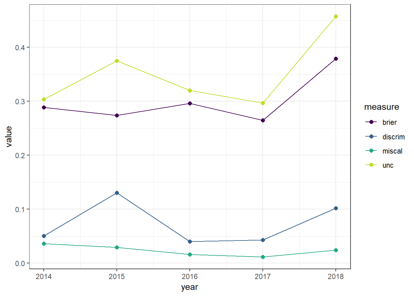

Interpreting this picture is a bit tricky. When looking at Brier scores, smaller values indicate better prediction. The same is true for miscalibration. Discrimination, on the other hand, is better when its higher. Uncertainty gives us an idea of how well the forecaster could do. Because the scales are different, I recommend looking at this next plot instead:

library(ggplot2)
bind_rows(scottbrier14, scottbrier15, scottbrier16, scottbrier17, scottbrier18) %>% 
  bind_cols(tibble(year = 2014:2018)) %>% 
  tidyr::gather(discrim, miscal, brier, unc, key = "measure", value = "value") %>% 
  group_by(measure) %>% 
  mutate(value_scaled = scale(value)) %>% 
  ungroup() %>% 
  ggplot(aes(x = year, y = value_scaled, colour = measure)) + geom_line() + geom_point(size = 2) + 
  theme_bw() + scale_colour_viridis_d(end = .9)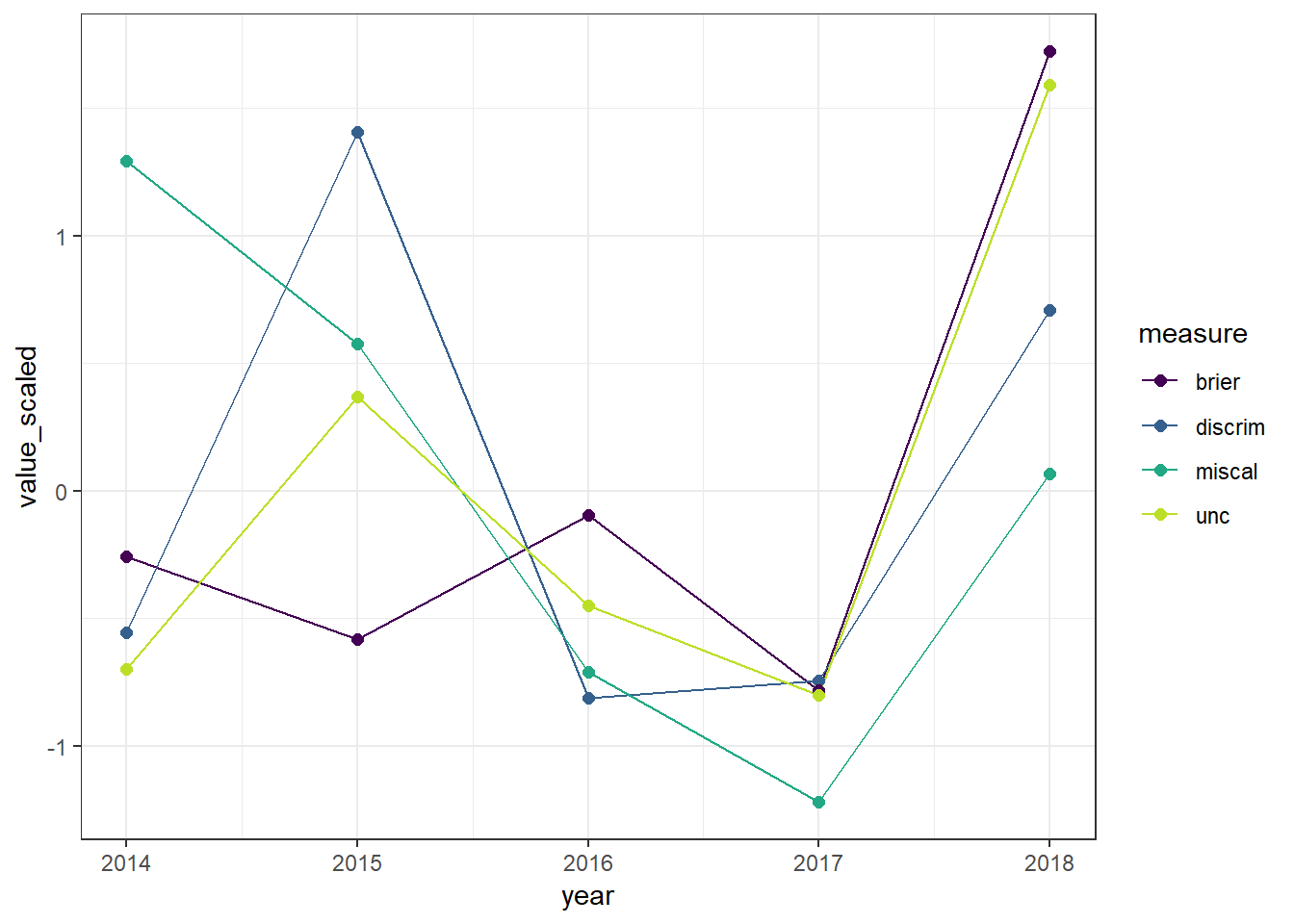

YMMV, but my reading of this is that 2018 was an odd year for Scott. He chose a set of events that had substantially more variation in the past, and while he did well at discriminating, he was also more miscalibrated than he’s been in the past. This lead to a much higher Brier score than he usually sees. Prior to that, his aggregate Brier score had been stable despite quite a bit of variation in the components.

Caveats

This brings us to the issue of data generation. While there are plenty of concerns with this exercise (correlation between events being a big one), Scott is also consciously choosing which events to make forecasts on. In the canonical examples for which Brier scores were developed (weather forecasting), the forecaster doesn’t get to pick and choose. So it becomes hard conceptually to interpret the Uncertainty score. Scott chooses the playing field for this game, so he gets to determine if he wants to make predictions on high-uncertainty events or low uncertainty events. Or at least he gets to do this based on his estimated probabilities. This means that his forecast accuracy effects the aggregate uncertainty in the events, insofar as Scott chooses which events to predict based on his forecasts and a desire to have a certain number of events in each bin.

I’ll have to think about this more to decide how it should impact our interpretations of Scott’s scores. I think it would help for Scott to provide details about his process for choosing which events to make forecasts about. I’m reasonably certain its changed the longer he’s done this project, so understanding that could help us understand why 2018 was such an odd-looking year.

Data scraping function

This is the function I used to scrape the results from Scott’s webpage. It’s kinda kludgy in a few places because Scott wasn’t 100% consistent in how he coded things. (e.g., He used colors rather than strike-through in 2014, and he didn’t always include line breaks between predictions.) But as far as I can tell, it works properly.

get_scotts_results <- function(url){
  
  
  if(sum(c("dplyr", "stringr") %in% (.packages())) < 2){
    stop("Function requires dplyr and stringr packages to be loaded")
  }
  
  webpage <- xml2::read_html(url)
  posttext_html <- rvest::html_nodes(webpage,'.pjgm-postcontent')
  tb <- posttext_html %>% as.character() %>% 
    str_split( "<br>|</p>\n<p>|6\\. Rep|30\\. 2014|>7\\. Demo|>32\\. HPM")
  
  tb[[1]] %>% as_tibble() %>% 
    mutate(wrong = str_extract(value, "<s>|</font>"),
           probbin = str_extract(value, ": \\d{2}")) %>% 
    filter(!is.na(probbin)) %>% 
    mutate(prob_chr = str_extract(probbin, "\\d{2}"),
           prob = as.numeric(prob_chr)/100,
           right = is.na(wrong),
           question = str_remove_all(value, "\\n|<s>|</s>")) %>% 
    select(question, prob, right)
  
}

And as long as we’re here, if you want to read more about Brier scores and the scoring package I used, here is a relevant article.